New Zealand Industry In Data
10 JUL 2025
Summary
The goal of this project is to go from online data source to reasonable visualisation of the most outstanding features of the data, via an exploration of the data using our standard tool set. Our standard for determining whether the data exploration is complete will be that the visualisation is both reasonable, and holds up to scrutiny by third parties.
We will choose a dataset based on it being conveniently available, and it being in a known file format that is easy to process. Economic data published by the New Zealand government provides a ready source of data matching these criteria.
We will attempt to conduct meaningful exploration of our chosen data set, create appropriate visualisations, and then draw conclusions based on mathematical analysis of the data.
Contents
- Summary
- Contents
- Problem
- Data
- Method
- Solution
- Results
- Next Steps
- Conclusion
Problem
When we come to dataset with pre-conceived notions about what that dataset contains, we risk losing the opportunity to gain real insights from the data itself.
How do we understand a complex data set without relying on the summaries and opinions of others (statisticians, researchers and data scientists)? How do we tease out the structure of the data while relying solely on the data itself?
Data
Source: Stats NZ - Large Datasets
File: Annual enterprise survey: 2024 financial year (provisional) – CSV
Method
-
Launch IDLE from virtual environment where Pandas and NumPy are installed.
PS C:\Projects\claude> .venv\scripts\activate
(.venv) PS C:\Projects\claude> python.exe -m idlelib.idle
-
Import Dependencies: Pandas, Statistics, MatPlotLib
>>> import pandas as pd
>>> import statistics as stats
>>> import matplotlib.pyplot as plt
-
Load dataset
>>> url = 'https://www.stats.govt.nz/assets/Uploads/Annual-enterprise-survey/Annual-enterprise-survey-2024-financial-year-provisional/Download-data/annual-enterprise-survey-2024-financial-year-provisional.csv'
>>> data = pd.read_csv(url)
-
Sanity Check
>>> data.shape
(55620, 10)
>>> data.head()
-
Set Max Columns to display for better view
>>> pd.set_option("display.max_columns", 20) >>> data.head() -
Count the number of occurrences of each data value in each column. This also gives us the relative frequency of each value.
>>> data_columns = data.columns >>> data_columns ... Index(['Year', 'Industry_aggregation_NZSIOC', 'Industry_code_NZSIOC', 'Industry_name_NZSIOC', 'Units', 'Variable_code', 'Variable_name', 'Variable_category', 'Value', 'Industry_code_ANZSIC06'], dtype='object') >>> for item in data_columns: print(item, data[item].value_counts()) -
Count the number of industries by name
>>> len(total_income['Industry_name_NZSIOC'].unique())
>>> # Array has 119 elements
N.B.: This can be amended to 118 industry categories. "Food product manufacturing" is not a proper category; "Food Product Manufacturing" is the actual category
-
Select rows denoting Total Income
>>> total_income = data.loc[data['Variable_name'] == 'Total income']
-
Remove commas from "Value" column so that the Object data type can be cast to Int
>>> total_income['Value'] = total_income['Value'].str.replace(',', '').astype(int) -
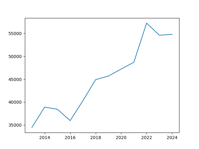
Sample Agriculture series data
>>> agriculture = total_income[total_income['Industry_name_NZSIOC'] == 'Agriculture, Forestry and Fishing']
-
It is linear regression time! Create linear regression and evaluate slope.
>>> agriculture_lr = stats.linear_regression(agriculture['Year'], agriculture['Value'])
>>> print(agriculture_lr)
-
Visualise to validate
>>> import matplotlib.pyplot as plt
>>> fig, ax = plt.subplots()
>>> ax.plot(agriculture['Year'], agriculture['Value'])
>>> plt.show()
Solution
-
For each "Industry_name_NZSIOC" (Column 3), capture the "Value" (Column 8) of "Variable_name" Total Income (Column 6) for each "Year" (Column 0).
>>> total_income = data.loc[data['Variable_name'] == 'Total income', 'Year', 'Industry_name_NZSIOC', 'Value']
-
For each subset of data captured above, calculate the linear regression of "Value" (Column 8). If the slope is positive, the industry is in a growth trend, if the slope is negative, the industry is in a contraction trend.
-
Graph 20 largest industries per 2024 "Value"
by highest and lowest slope. -
Graph all industries in a negative growth trend (contracting)
Code
from datetime import datetime

timestamp = datetime.now().isoformat(timespec='seconds')

# Initialise dictionary where industry growth / contraction is kept
industry_trends = {}

print(f'Starting imports ({timestamp})...')

# Principal imports
import pandas as pd
import statistics as stats
import matplotlib.pyplot as plt

# Load data set from web or local file path as appropriate
url = 'https://www.stats.govt.nz/assets/Uploads/Annual-enterprise-survey/Annual-enterprise-survey-2024-financial-year-provisional/Download-data/annual-enterprise-survey-2024-financial-year-provisional.csv'
local_file_path = 'annual-enterprise-survey-2024-financial-year-provisional.csv'
timestamp = datetime.now().isoformat(timespec='seconds')
print(f'Loading data set ({timestamp}):', local_file_path, sep='\n')
data = pd.read_csv('annual-enterprise-survey-2024-financial-year-provisional.csv')
print('Sanity check: data.shape', data.shape)

# Total income subset: Select rows denoting Total Income
total_income = data.loc[data['Variable_name'] == 'Total income']

# Remove commas from "Value" column so that the Object data type can be cast to Int
total_income['Value'] = total_income['Value'].str.replace(',', '').astype(int)

# Query for top industries based on 2024 total income
income_2024 = total_income.query('Year == 2024 and Variable_name == "Total income"')
industries_sorted = income_2024.sort_values(by=['Value'], ascending=False)
# Exclude 'All industries', which is at the top of the sorted list
top_industries = industries_sorted.head(20)[1:]

# Set up graphical representation of contracting industries
fig, ax = plt.subplots()

# Loop through industries and select that industry as a subset
for industry in total_income['Industry_name_NZSIOC'].unique():
    industry_subset = total_income.query(f'Industry_name_NZSIOC == "{industry}"')
    print('industry_subest.shape:', industry_subset.shape)
    industry_subset_x = industry_subset["Year"]
    industry_subset_y = industry_subset["Value"]
    try:
        industry_subset_lr = stats.linear_regression(industry_subset_x, industry_subset_y)
    except Exception as e:
        print(f"Industry {industry} encountered exception.")
        print(f"Exception of type {type(e)}:", str(e), sep='\n')
    else:
        print(f'Industry: {industry}\nLinear regression slope: {industry_subset_lr.slope}, intercept: {industry_subset_lr.intercept}')
        trend = 'growing' if industry_subset_lr.slope > 0 else 'contracting'
        print(f'The {industry} industry growth trend is ', trend, '.', sep='')
        industry_trends.update({industry: trend})
        # Conditional add to graphical representation of contracting industries
        if trend == 'contracting':
            ax.plot(industry_subset_x, industry_subset_y, label=industry)

# Labelling on graphical representation of contracting industries
ax.set_ylabel('Year')
ax.set_ylabel('Million NZ Dollars')
ax.set_title("NZ Contracting Industries")
ax.legend()
plt.show()

# Graph top industries (in growth trend)
fig, ax = plt.subplots()

for industry in top_industries['Industry_name_NZSIOC']:
    industry_trends.update({industry: "growing"})
    industry_subset = total_income.query(f'Industry_name_NZSIOC == "{industry}"')
    industry_subset_x = industry_subset["Year"]
    industry_subset_y = industry_subset["Value"]
    ax.plot(industry_subset_x, industry_subset_y, label=industry)

# Labelling on graphical representation of top industries
ax.set_ylabel('Year')
ax.set_ylabel('Million NZ Dollars')
ax.set_title("NZ Top Industries (2024)")
ax.legend()
plt.show()

# Output the winners (to 20) and losers (all in downward trend)
top_20_names = list(top_industries['Industry_name_NZSIOC'])
# print('Top 20 Names:', top_20_names, '\n')
print('='*10, 'Trends Dictionary', sep='\n')
for ind, tre in industry_trends.items():
    if tre == 'contracting' or ind in top_20_names:
        print(ind, "is in a", tre, "trend")

# That is a wrap
timestamp = datetime.now().isoformat(timespec='seconds')
print(f'Ending at {timestamp}')
Results
Industries in a growth trend
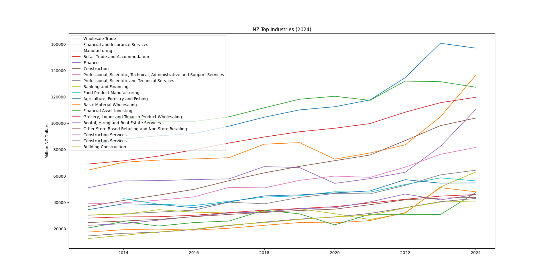
(Click for larger version)
Industries in a contraction trend
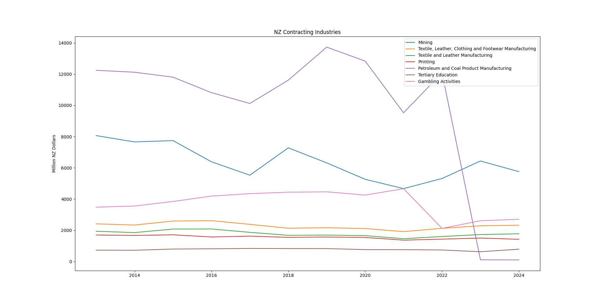
(Click for larger version)
Next Steps
-
Output top 20 and contracting industries to dataframe for ranking and tabular display
-
Generalise script to work with different data sources
Conclusion
Aggregating creativity and tradition, we are able to get the data to speak for itself.
We chose a dataset based on its availability and file format. Understanding what data is contained in the set required concerted efforts at data exploration. The first most useful data subset we discovered was year-on-year growth or decline for a broad range of New Zealand industries. We were able to plot this data, and then make rule-of-thumb determinations as to which industries were growing and which were in decline (slope of linear regression), in terms of New Zealand dollars (total income).
There most certainly exists a more elegant solution than the many steps described here. The priviledge of finding the yet-more-elegant-solution is the pervue of the mathematician, the data scientist, the computer scientist, the thinker, the ponderer.